Lab 10 - Localization (Simulation)
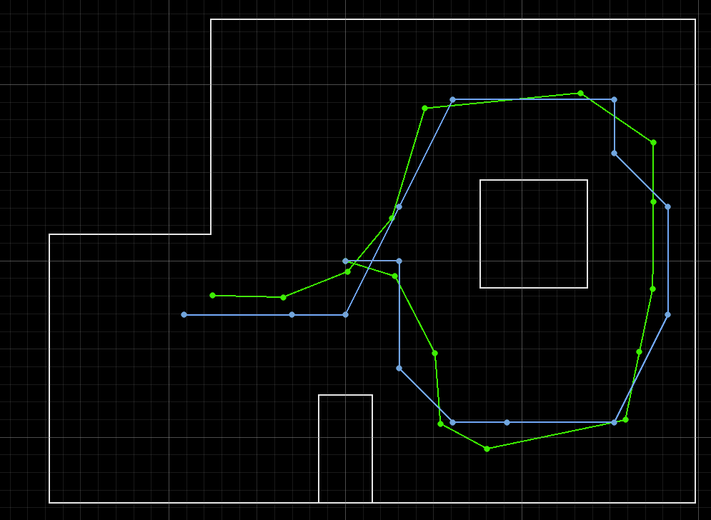
The objective of Lab 10 is to implement the Bayes Filter into the simulator to perform grid localization.
Prelab
The prelab of this lab consists of reviewing a few aspects that will be useful for the lab:
-
The world will be discretized into a finite 3D grid space, where the axis represent $x$, $y$, and $\theta$. There are 20x20x18 cells in total, and each cell will contain the probability that the robot is in that state.
-
The sensor and odometry model used, as well as the Bayes Filter are explained in the following sections.
Bayes Filter
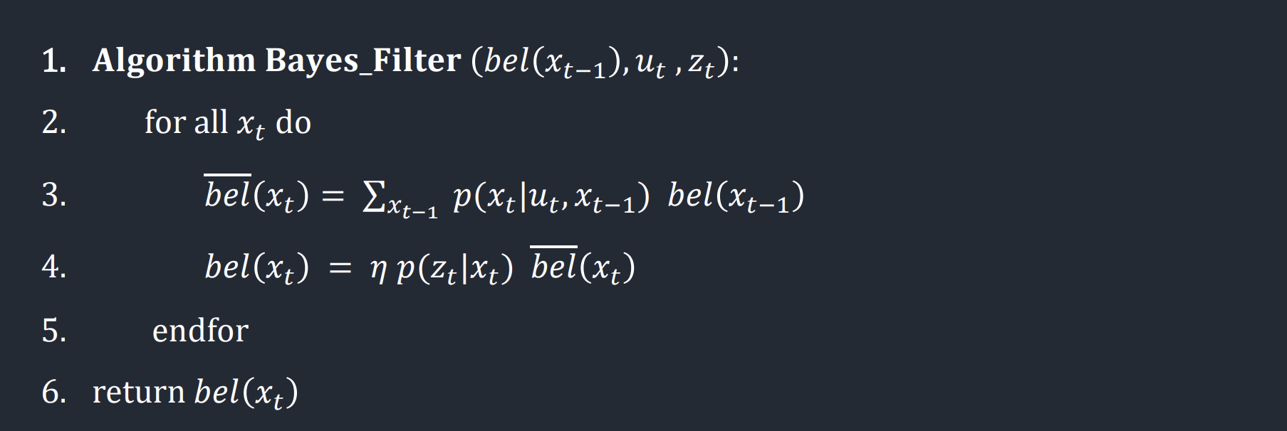
The goal of this lab is to implement the Bayes Filter into the simulator. The Bayes Filter has two steps: a prediction step, where we obtain the prior beliefs (bel_bar) that we get to a certain state, given a previous state, for all states; and an update step, that updates the belief that we are in certain state given the probability of obtaining a sensor reading and the prior belief that we are in certain state, for all states. The Bayes Filter pseudo-code, from Lecture, is the following:
1. Compute Control
For the Prediction Step, we need the probability given by the odometry model. This model, however, needs a current pose (or state), a previous one, and a control. The control needs to be extracted from the odometry readings, and consists of an initial rotation, a translation, and a final rotation.
1
2
3
4
5
6
7
8
9
10
11
12
13
14
15
16
17
18
19
20
21
def compute_control(cur_pose, prev_pose):
    """ Given the current and previous odometry poses, this function extracts
    the control information based on the odometry motion model.

    Args:
        cur_pose  ([Pose]): Current Pose
        prev_pose ([Pose]): Previous Pose

    Returns:
        [delta_rot_1]: Rotation 1  (degrees)
        [delta_trans]: Translation (meters)
        [delta_rot_2]: Rotation 2  (degrees)
    """
    delta_rot_1 = np.degrees(np.arctan2(cur_pose[1]-prev_pose[1], cur_pose[0]-prev_pose[0])) - prev_pose[2]
    delta_trans = np.sqrt((cur_pose[0]-prev_pose[0])**2 + (cur_pose[1]-prev_pose[1])**2)
    delta_rot_2 = cur_pose[2] - prev_pose[2] - delta_rot_1

    delta_rot_1 = mapper.normalize_angle(delta_rot_1)
    delta_rot_2 = mapper.normalize_angle(delta_rot_2)

    return delta_rot_1, delta_trans, delta_rot_2
Note that the arctan returns radians, which need to be transformed to degrees. Additionally, all angles are then normalized to $[-180º,+180º)$.
2. Odometry Model
The Odometry Model is responsible for returning the probability of arriving to a current pose, given a previous pose and a control action. This model can be represented as a gaussian curve with some noise, where the mean is the actual control used to get from the previous pose to the current one. Then, the model returns the probability of the desired control given the actual control. As the control contains three terms (rotation, translation, rotation), we need to compute the three probabilities, and return the product.
1
2
3
4
5
6
7
8
9
10
11
12
13
14
15
16
17
18
19
20
21
22
23
def odom_motion_model(cur_pose, prev_pose, u):
    """ Odometry Motion Model

    Args:
        cur_pose  ([Pose]): Current Pose
        prev_pose ([Pose]): Previous Pose
        (rot1, trans, rot2) (float, float, float): A tuple with control data in the format
                                                   format (rot1, trans, rot2) with units (degrees, meters, degrees)


    Returns:
        prob [float]: Probability p(x'|x, u)
    """

    actual_u = compute_control(cur_pose, prev_pose)

    prob1 = loc.gaussian(u[0], actual_u[0], loc.odom_rot_sigma)
    prob2 = loc.gaussian(u[1], actual_u[1], loc.odom_trans_sigma)
    prob3 = loc.gaussian(u[2], actual_u[2], loc.odom_rot_sigma)

    prob = prob1*prob2*prob3

    return prob
3. Prediction Step
The Prediction Step consists of updating the values of the prior belief for every step, given the current and previous odometry readings. For this step, we need the belief that we were in certain state (bel), and the probability that we moved from that state to a new one, given by the odometry model. For each new state, we need to consider all previous steps. Additonally, we have to compute the prior beliefs for all new states.
1
2
3
4
5
6
7
8
9
10
11
12
13
14
15
16
17
18
19
20
21
22
23
24
25
26
27
def prediction_step(cur_odom, prev_odom):
    """ Prediction step of the Bayes Filter.
    Update the probabilities in loc.bel_bar based on loc.bel from the previous time step and the odometry motion model.

    Args:
        cur_odom  ([Pose]): Current Pose
        prev_odom ([Pose]): Previous Pose
    """

    u = compute_control(cur_odom, prev_odom)

    loc.bel_bar = np.zeros((mapper.MAX_CELLS_X, mapper.MAX_CELLS_Y, mapper.MAX_CELLS_A))


    for i_x in range(mapper.MAX_CELLS_X):
        for i_y in range(mapper.MAX_CELLS_Y):
            for i_theta in range(mapper.MAX_CELLS_A):
                prev_pose = mapper.from_map(i_x, i_y, i_theta)

                if  loc.bel[i_x][i_y][i_theta] >= 0.0001:

                    for j_x in range(mapper.MAX_CELLS_X):
                        for j_y in range(mapper.MAX_CELLS_Y):
                            for j_theta in range(mapper.MAX_CELLS_A):
                                cur_pose = mapper.from_map(j_x, j_y, j_theta)
                                prob_j =  odom_motion_model(cur_pose, prev_pose, u)
                                loc.bel_bar[j_x][j_y][j_theta] = loc.bel_bar[j_x][j_y][j_theta] + prob_j*loc.bel[i_x][i_y][i_theta]
To improve computation time, all those states whose belief is small (<0.0001) won’t be considered.
4. Sensor Model
Once we have obtained the previous beliefs for every state, we need to incorporate the sensor readings. The Update Step incorporates the prior belief (bel_bar) that we are in certain state, given the sensor readings, into the final belief (bel). The Sensor Model, therefore, returns the probability to obtain a certain reading (obs_range_data) given a state (obs). For each state, there are 18 sensor readings, correspondign to each turn of the robot. The Sensor Model returns 18 probabilities, corresponding to those turns. The Sensor Model is a gaussian model, with a certain sensor noise, similar to the one used for the odometry model.
1
2
3
4
5
6
7
8
9
10
11
12
13
14
15
16
17
def sensor_model(obs):
    """ This is the equivalent of p(z|x).


    Args:
        obs ([ndarray]): A 1D array consisting of the true observations for a specific robot pose in the map

    Returns:
        [ndarray]: Returns a 1D array of size 18 (=loc.OBS_PER_CELL) with the likelihoods of each individual sensor measurement
    """

    prob_array = np.zeros(mapper.OBS_PER_CELL)

    for i in range(mapper.OBS_PER_CELL):
        prob_array[i] = loc.gaussian(loc.obs_range_data[i], obs[i], loc.sensor_sigma)

    return prob_array
5. Update Step
Last, we need to update the belief for every state given the probability of that state (from the sensor model), and the prior beliefs (bel_bar). As mentioned before, the Sensor Model returns 18 probabilities for each state. We will use the product of all of them to compute the belief for every state.
1
2
3
4
5
6
7
8
9
10
11
12
13
def update_step():
    """ Update step of the Bayes Filter.
    Update the probabilities in loc.bel based on loc.bel_bar and the sensor model.
    """

    for i_x in range(mapper.MAX_CELLS_X):
        for i_y in range(mapper.MAX_CELLS_Y):
            for i_theta in range(mapper.MAX_CELLS_A):
                obs = mapper.get_views(i_x, i_y, i_theta)
                prob_sensor =  np.prod(sensor_model(obs))
                loc.bel[i_x][i_y][i_theta] = prob_sensor*loc.bel_bar[i_x][i_y][i_theta]

    loc.bel = loc.bel / np.sum(loc.bel)
Note how after every update step, all beliefs are normalized to sum up to 1.
Simulation
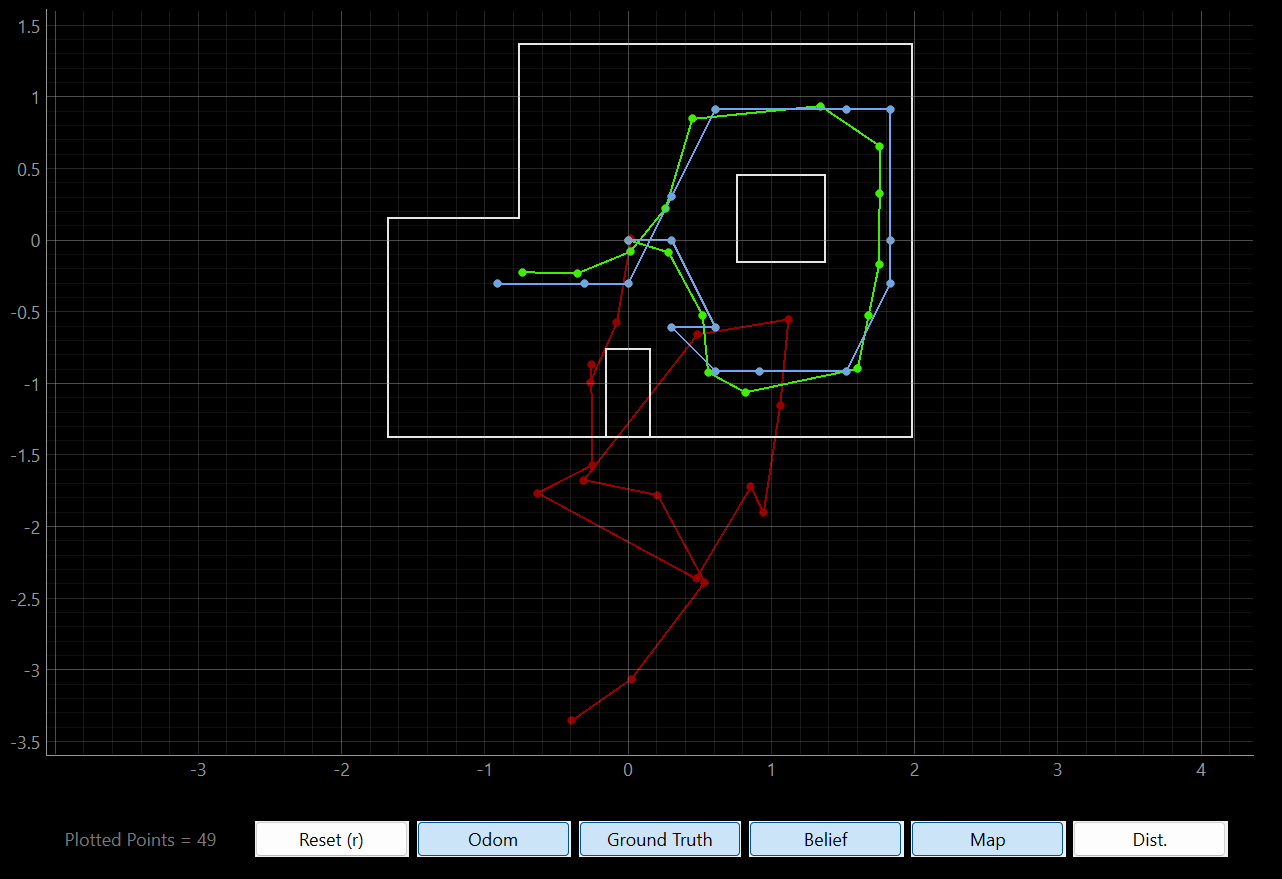
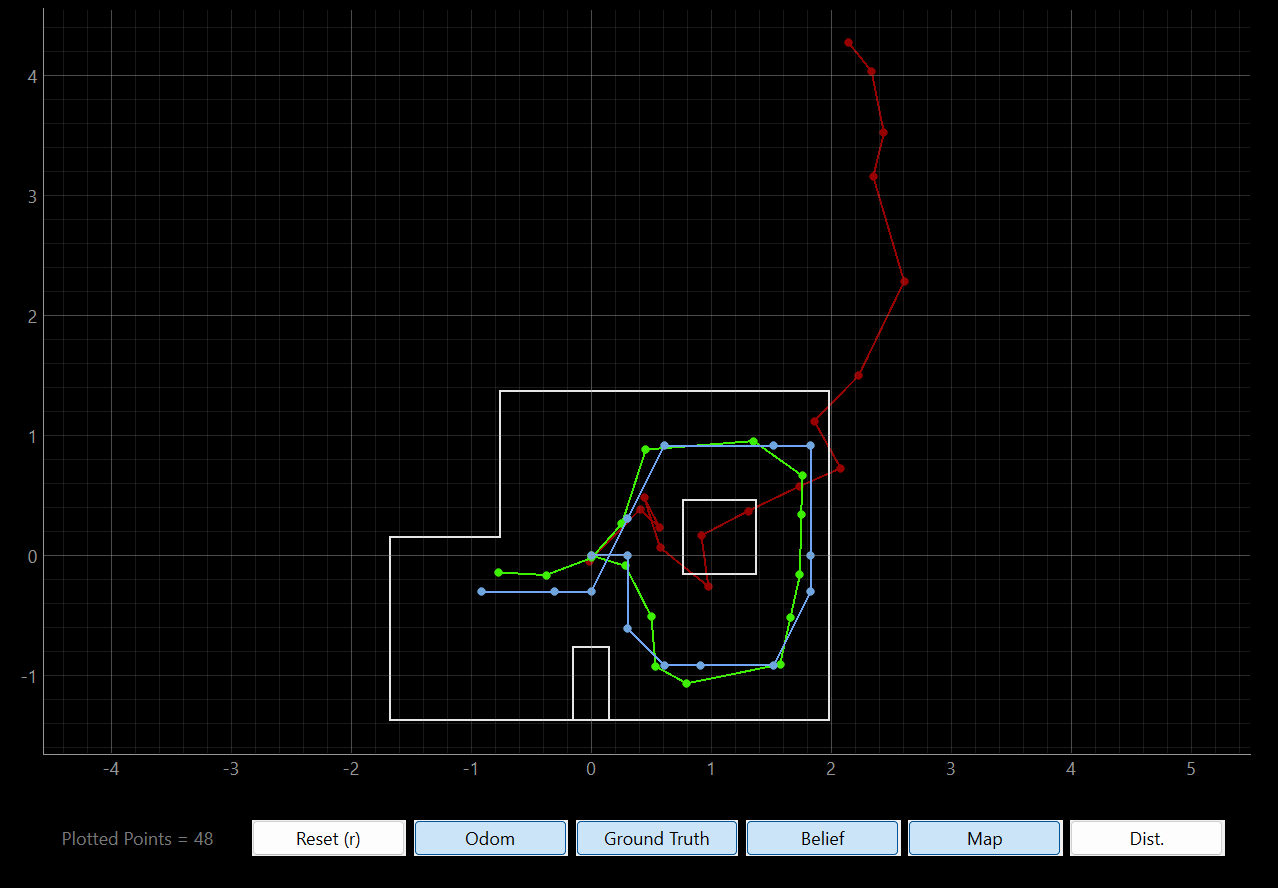
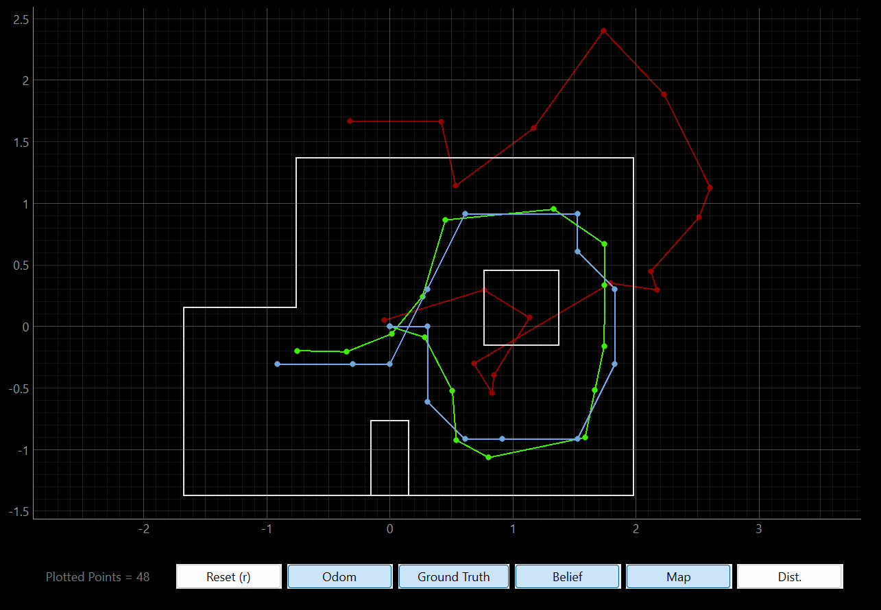
Now that we have implemented the Bayes Filter, it’s time to perform a simulation. The codebase already includes the map and the trajectory of the robot. Running the simulation we can see that the Bayes Filter is quite robust in predicting the localization of the robot, and following its path, with slight error. The results of three different runs are shown below. We can see that the Filter is consistent across runs.
| Run #1 | Run #2 | Run #3 |
 |
 |
 |
Here is a video of the simulation running.
References
The code for this lab was inspired from the class lectures (16, 17, 18), and the TA’s websites (Larry, Ignacio, Julian, Liam, and Rafi).