Lab 2 - IMU

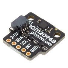
The objective of Lab 2 is to learn how to use the IMU; sampling data from the Accelerometer and from the Gyroscope.

Prelab

The prelab for Lab 2 consists on reading through the data sheet of the IMU.

Tasks

1. IMU Set Up

To setup the IMU we need to install the SparkFun 9DOF IMU Breakout - ICM 20948 - Arduino Library. After that, we will run the Example 1, Basics, from the library examples. The value AD0_VAL represents the last bit of the I2C address. As the jumper in my IMU is closed, its value should be set to 0. Additionally, to indicate that the board is running, I will add a small loop that blinks the LED 3 times.

1
2
3
4
5
6
7
pinMode(LED_BUILTIN, OUTPUT);

for(int i=0; i<3; i++){
    digitalWrite(LED_BUILTIN, HIGH);
    delay(1000);
    digitalWrite(LED_BUILTIN, LOW);
    delay(1000);

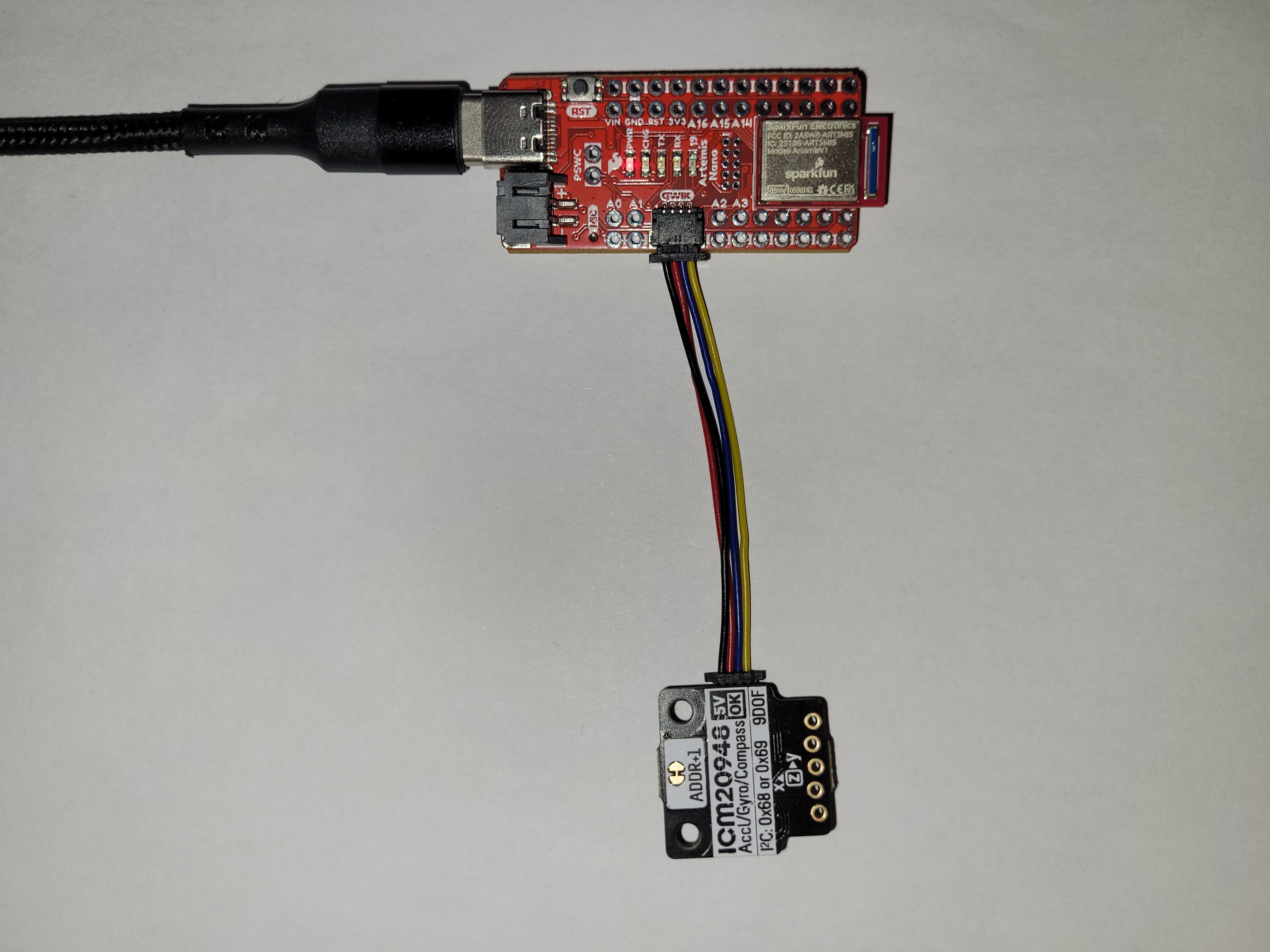
In the video below we can see that the IMU is recording data from the accelerometer, gyroscope and magnetometer. The accelerometer displays the acceleration in the three axis in mg (mili-g), while the gyroscope displays the angular velocity in the three axis in degrees per second.

2. Accelerometer

We want to convert the accelerometer data into pitch and roll. To do this, I will use the equations from class. The method used to reocord data will be explained later in Task 4.

1
2
pitch_a = atan2(myICM.accX(), myICM.accZ())*180/M_PI;
roll_a = atan2(myICM.accY(), myICM.accZ())*180/M_PI;

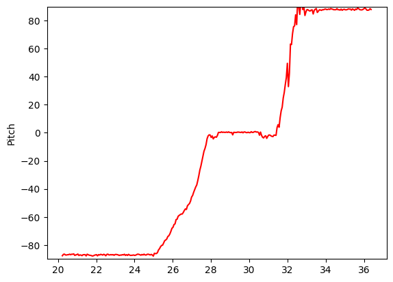
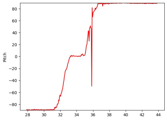
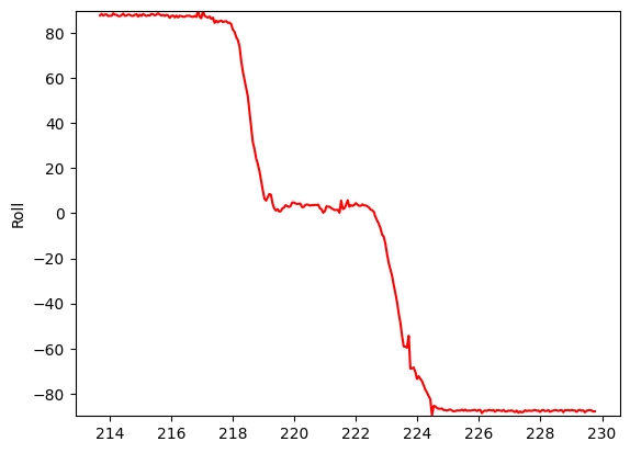
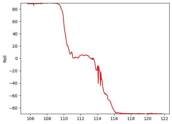
Testing the roll, the output at both ends -88.5 and 88.3. I will add to the calculations a 90/88.5 conversion factor, so that real 90º correspond to 90º measurements. I repeated the same test for the pitch, where the output at both ends was 88.6 and -87.87; so the conversion factor added is 90/88.6. We can notice that after the calibration, both ends are much closer to +/-90º.

Before calibration	Output at both ends	After calibration

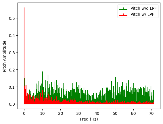
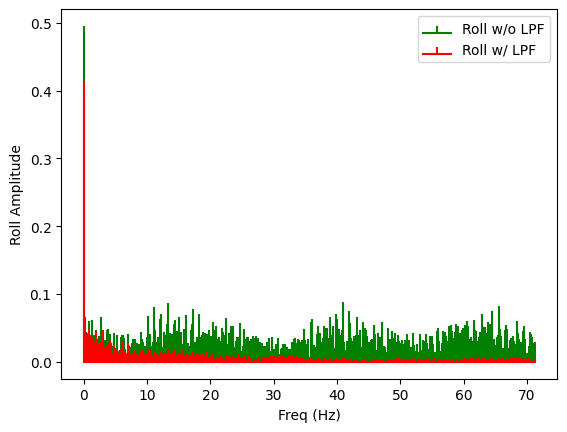
The FFT shows some noise in the higher frequencies. However, it is not too large. This is because the IMU has a Low Pass Filter already implemented, according to the datasheet. Nevertheless, I will use a Low Pass Filter, following the equations from the class slides. The same equations are used to filter the roll. With a sample rate of approximately 0.007 and a cut-off frequency of around 3Hz or 4Hz, we obtain that alpha is 0.14. A downside to the LPF is a slight delay, which can be improved with data from the gyroscope.

1
2
pitch_a_LPF[n] = alpha*pitch_a + (1-alpha)*pitch_a_LPF[n-1];
pitch_a_LPF[n-1] = pitch_a_LPF[n];

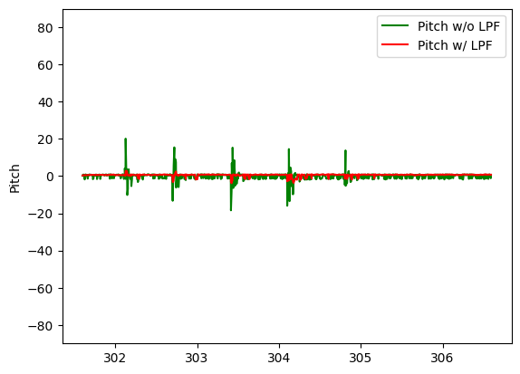
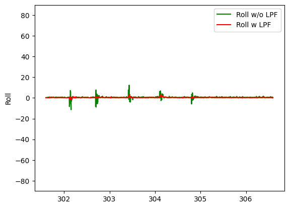
Even though there’s already a LPF in the chip, we can see that by applying a LPF the noise is reduced considerably.

Without LPF	With LPF

3. Gyroscope

The gyroscope can also be used to obtain pitch and roll, as well as yaw. We can use the following equations, where we integrate the data recorded (angular velocity) to obtain angles.

1
2
3
pitch_g = pitch_g + myICM.gyrX()*dt;
roll_g = roll_g - myICM.gyrY()*dt;
yaw_g = yaw_g + myICM.gyrZ()*dt;

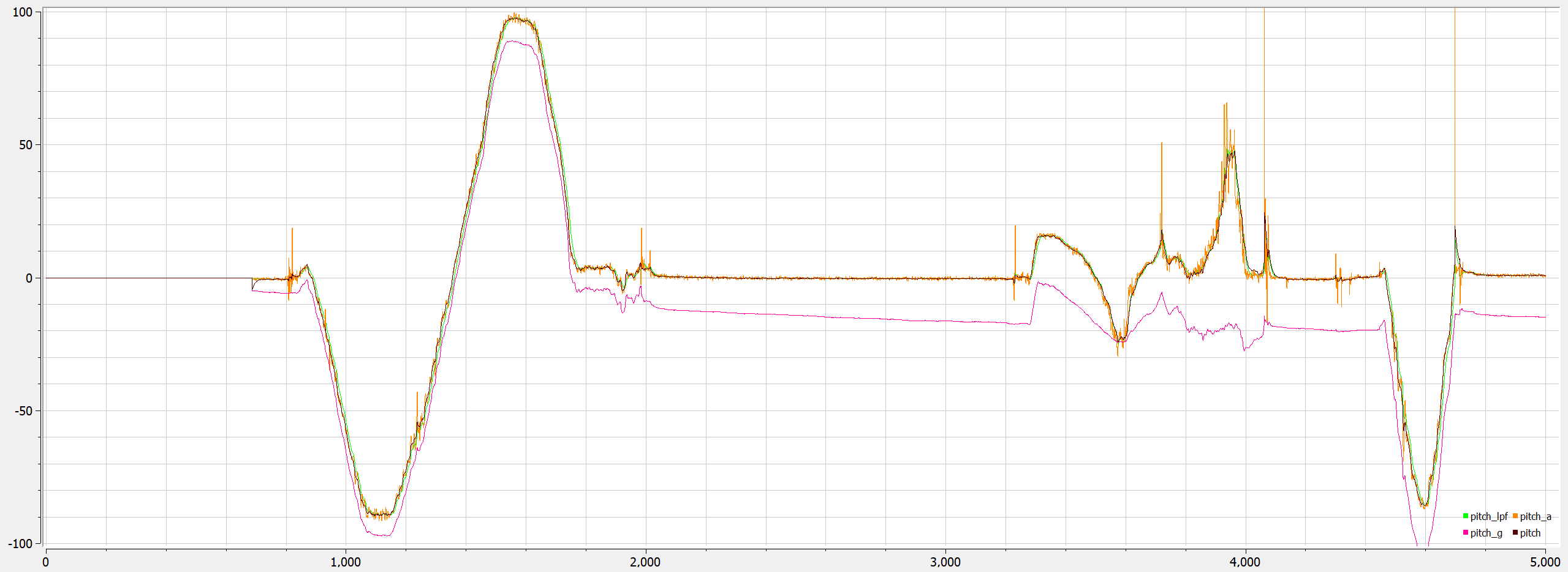
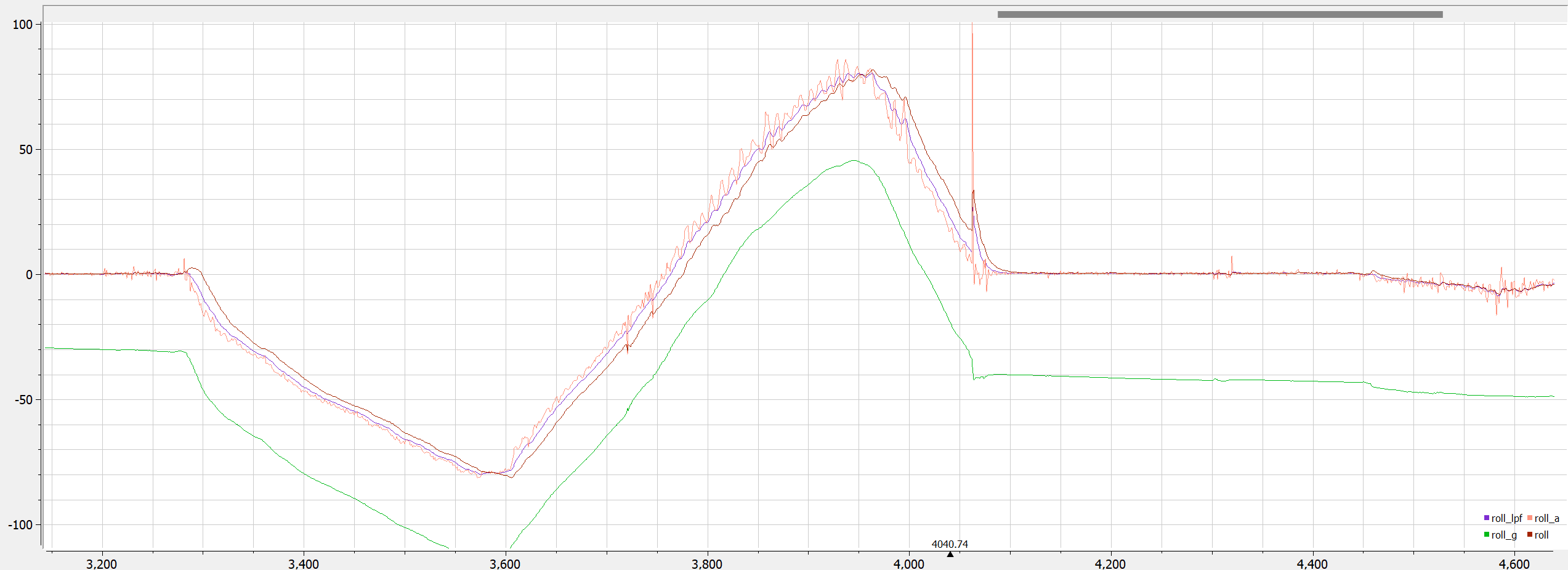
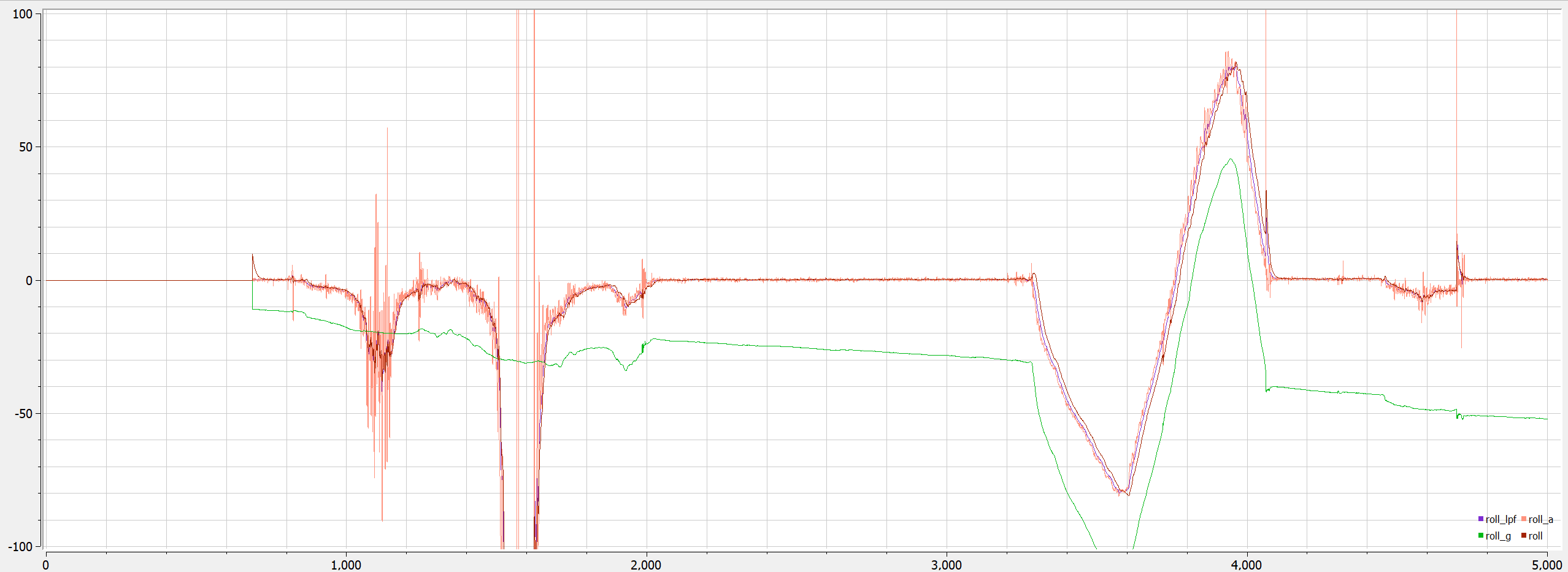
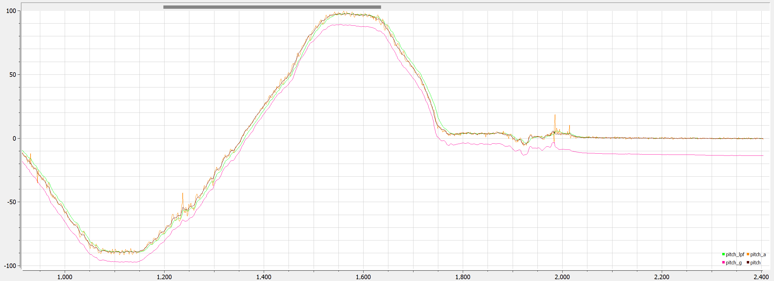
If we compare the results with those from the acceleromter, we can notice that they have less noise, but are susceptible to drift: the signal increases over time.

Using a complimentary filter can help us get more accurate results. This filter takes into account both the results from the accelerometer and the gyroscope, getting rid of noise and drift.

1
2
pitch = (pitch+myICM.gyrX()*dt)*(1-alpha_cf) + pitch_a*alpha_cf;
roll = (roll+myICM.gyrY()*dt)*(1-alpha_cf) + roll_a*alpha_cf;

We can see the results in this comparison, where we display pitch and roll from the accelerometer, with LPF, from the gyroscope, and from the complimentary filter. I recommend opening each image in a new window to see the different signals.

Whole signal	Zoomed in view

4. Data Sampling

To make sure that the main loop runs as fast as possible I created some flags (start_recording, send_data) that enable certain sections of the main loop to run, and will be updated with commands. The rest is executed inside the main loop, so we can check for new data available faster. The structure of the code is similar to the one below.

1
2
3
4
5
6
7
8
9
10
11
12
13
14
15
16
17
18
19
20
21
22
23
24
25
26
/*Command example definition*/
case START_RECORDING:{
    start_recording = true;
    i=0;
    break;}
/*Other commands*/

/*main loop*/
while (central.connected()) {        
    write_data();

    if(start_recording == true){
        if (myICM.dataReady()){
            myICM.getAGMT(); //Obtain data

            /*Do calculations*/
            /*Store in array*/

            i++;
        }
    }

    /*Other flags/ifs*/

    read_data();
}

With this implementation, we can sample new data, on average, every 5 ms. The data is stored in float types, as they are precise enough for our measures, but don’t occupy too much memory. Each data will be stored in their own array inside the Artemis so they are easier to work with, but will be sent over Bluetooth on a single string.

If we consider the case where we want to obtain pitch, roll and yaw from with the complimentary filter, we will have to store 4 floats every time (time stamps should be included). A float is 4 bytes, so each point will be 16 bytes. The Artemis has 384kB of RAM, so we will be able to store approximately 24000 data points. This means we can theoretically capture up to 120 seconds of data. However, we cannot expect the whole RAM to be filled with this arrays, as there will be a stack overflow. What we can assure is that we can capture 5 seconds of data. For the following data recordings, we recorded 2000 points, with a time difference of 8.23 seconds, yielding a 4.11 ms sampling rate.

Conclusion

In this lab we have learned how to use the accelerometer and gyroscope of the IMU. We have also learned how to filter the signals to obtain more accurate results. Last, we have learned how to implement the code in order for it to be fast.