Lab 7 - Kalman Filter

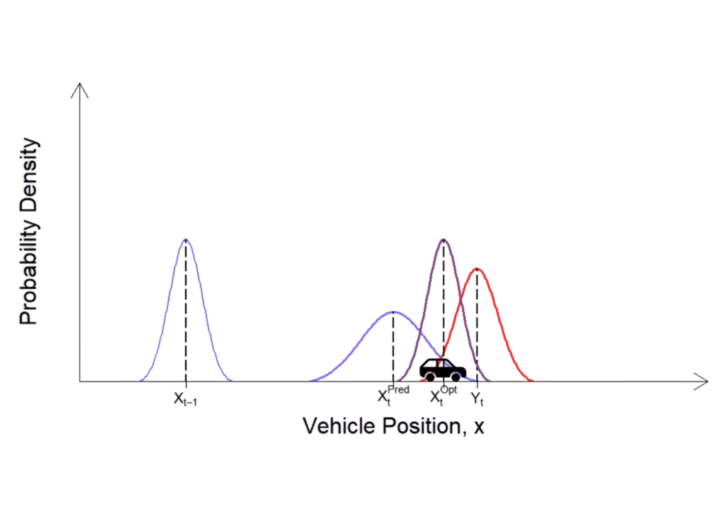
The objective of Lab 7 is to develop a Kalman Filter for our robot, and simulate in Python.

Prelab

There is no prelab for this lab.

Tasks

1. Drag and Momentum Estimation

The Kalman Filter needs a system model to work, given by the A and B matrices. These matrices are built with the drag and mass of the car, so we need to estimate those parameters. To do so, we perform a speed test, where the car moves forward towards a wall, and we record the distance and time stamps. The goal is that the car reaches a steady state speed, from which we can estimate the drag and mass. However, the ToF sensor only has a 4m range, so distances above that value are inaccurate. To ensure that we reach steady state, the car will run for an arbitrary amount of time, and then it will start recording data. When it gets to 0.5m to the wall, it will stop. The arbitrary waiting time, and the input to the motor is set with Bluetooth (id.wait_time and id.pid, respectively).

1
2
3
4
5
6
7
8
9
10
11
12
13
14
15
16
17
18
19
20
21
22
23
24
25
26
27
if(id.run_test){

  /*
   *  Obtain distance, dt, and error...
   */
        
  if(id.data_ready && ((id.curr_time - id.start_time) > id.wait_time)){
    /*
     *  Update values to send via Bluetooth if data ready, and waiting time ended...
     */
    id.i++;
  }
          
  if(id.i >= N_ID){
    /*
     *  If I run out of space, end test...
     */
  }

  if((id.error <= 5) && (id.i >= 1)){
    /*
     *  If I get too close to the wall, end test...
     */
  }

  setSpeed(id.pid, id.pid);
}

After trial and error, I obtained the following data, with a motor input of $u=80%$:

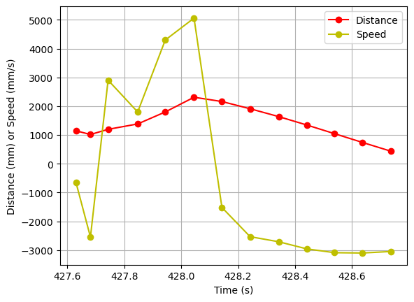
Note that the first values are unreliable, probably because the robot was still more than 4m away from the wall. Considering only the steady state section:

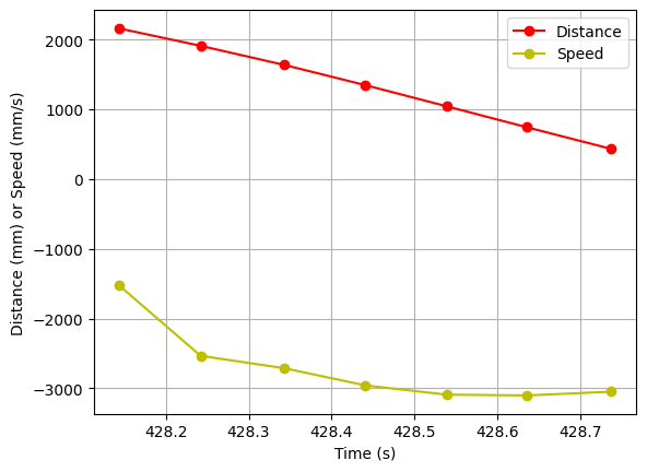
We find out that the steady state speed is $v_{ss}=3050mm/s$. The 90% value of this speed is 2745mm/s, corresponding to a time stamp of 428.343s. The test started at 425.933s, so the 90% rise time is $t_{90} = 2.41s$. The values for d and m are obtained using the equations from lecture:

2. Kalman Filter Initialization

The next step is to initialize the Kalman Filter. First, we have to compute the A, B and C matrices, given by:

Next, I have to discretize the A and B matrices. We can use the following equations. In my case, delta_t is the sampling time of the ToF sensor. As discussed in Lab 5, this sampling time is 100ms.

1
2
A_d = np.eye(2) + delta_t * A
B_d = delta_t * B

Last, we have to initialize the state vector, as well as the process and sensor noise.

State initialization:

1
2
x = np.array([[-distance_data[0]],[0]])
sigma = np.array([[1^2, 0] ,[0, 20^2]])

Noise initialization:

1
2
3
4
5
6
sigma_1 = np.sqrt((10**2)*1/delta_t)                ## Distance noise (from lecture)
sigma_2 = np.sqrt((10**2)*1/delta_t)                ## Speed noise (from lecture)
sigma_3 = 20                                        ## Measurement noise from TOF, approx 20mm

sigma_u = np.array([[sigma_1**2,0],[0,sigma_2**2]]) ## We assume uncorrelated noise, and therefore a diagonal matrix works.
sigma_z = np.array([[sigma_3**2]])

The values for sigma 1, 2 and 3, this first time, are an approximation, following the guidelines from lecture, and are based on the sampling time (which determines the process noise), and the ToF noise (which determines the sensor noise). These values will later be changed to adapt the Filter to the real values.

3. Kalman Filter Implementation

Last, we have to implement the Kalman Filter in Python. I performed a test where the robot approaches the wall, and recorded the values of distance, time, and motor input. The main code for the Filter was provided in the lab handout, but I made some adjustments so that it only updates the measurement prediction when a new measurement is available:

1
2
3
4
5
6
7
8
9
10
11
12
13
14
15
16
17
def kf(mu,sigma,u,y, new_reading):
    
    mu_p = A_d.dot(mu) + B_d.dot(u)                                        ## State prediction
    sigma_p = A_d.dot(sigma.dot(A_d.transpose())) + sigma_u                ## State prediction uncertainty
    
    if(new_reading):
        sigma_m = C.dot(sigma_p.dot(C.transpose())) + sigma_z              ## Measurement noise
        kkf_gain = sigma_p.dot(C.transpose().dot(np.linalg.inv(sigma_m)))  ## Kalman Filter Gain

        y_m = y - C.dot(mu_p)
        mu = mu_p + kkf_gain.dot(y_m)                                      ## New State
        sigma=(np.eye(2)-kkf_gain.dot(C)).dot(sigma_p)                     ## New State uncertainty
    else:
        mu = mu_p
        sigma = sigma_p

    return mu,sigma

Now, I have to loop through the recorded values and use the Kalman Filter to obtain the estimations. The loop will obtain a new estimation every 10ms. As readings are recorded every 100ms, we will have 10 predictions for every estimation. I will keep track of when a new reading is obtained. Additionally, I added some code so that the Kalman filter considers the first data point (which is in fact a new reading), a new reading correctly. The value of itime will be useful when plotting the results.

1
2
3
4
5
6
7
8
9
10
11
12
13
14
15
16
17
18
19
20
21
22
j = 0
first_time = 1

kfdistance = []
itime = []

for i in range(0, int(time_data[len(time_data)-1])-int(time_data[0]), 10):
    
    if(time_data[j+1] <= (i+int(time_data[0]))):
        j = j + 1
        new_reading = 1
    else:
        new_reading = 0

    if first_time:
        new_reading = 1
        first_time = 0

    x, sigma = kf(x, sigma, u_data[j]/100, -distance_data[j], new_reading)
    
    kfdistance.append(x[0])
    itime.append(i+int(time_data[0]))

4. Results

With the initial values of sigma we obtain the following results:

1. sigma_1 = 31.623; sigma_2 = 31.623; sigma_3 = 20

We can see that the Kalman filter reacts when a new reading is available, but is not very reliable when predicting values.

2. sigma_1 = 100; sigma_2 = 100; sigma_3 = 1

Now, we will add more noise to the process, but trust more the distance reading. The results don’t differ much.

3. sigma_1 = 1; sigma_2 = 1; sigma_3 = 100

If we distrust the readings, then the Kalman Filter deviates from the real values.

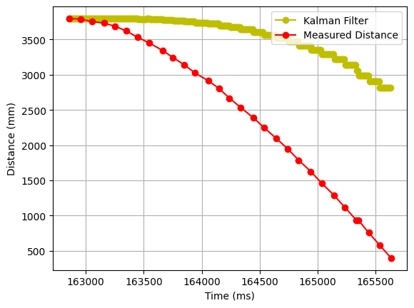
4. sigma_1 = 1; sigma_2 = 1; sigma_3 = 1

If we trust everything equally, we still have errors in the prediction values.

5. sigma_1 = 1; sigma_2 = 100; sigma_3 = 1

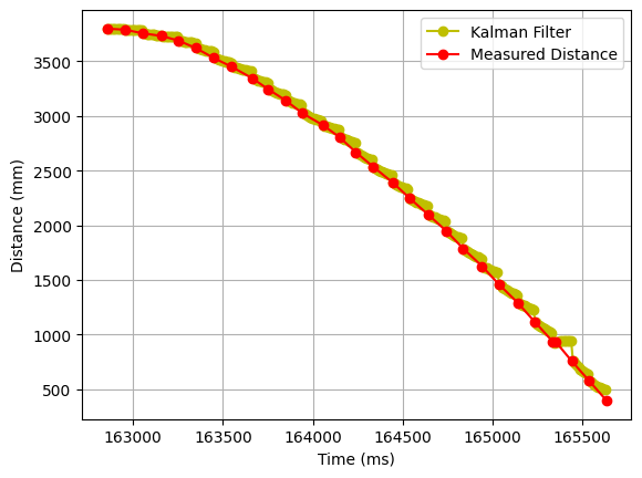
From the above tests, we can see that the speed is not predicted accurately. Therefore, I will increase its noise, but rely on the sensor reading and the distance prediction. This time, the Kalman Filter works pretty good.